
Filtering Data
A filter hides the rows that do not match a condition and keeps the rest, without deleting anything. In Excel select the table and choose Data > Filter (Ctrl+Shift+L); small arrows appear in the header row so you can pick values to keep. The first row must hold headers.
The FILTER(range, condition) function does the same in a formula. The condition is a test on a column, such as C2:C6>20, and the matching rows spill below the formula.
In Excel: click a cell in the table and press Ctrl+Shift+L. A small arrow appears in each header cell. Open the arrow on the Group column to choose which values to keep.
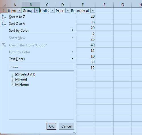
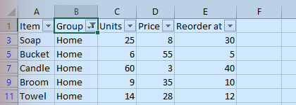
With only Home ticked, the other rows are hidden (not deleted). The status bar at the bottom reads "5 of 10 records found".
Does filtering delete the hidden rows?
Keep only the rows where the Group in column B is Home, starting in F2.
Finish the quick check (and any code exercise) to complete this lesson, or mark it done yourself.
Tip: use the left and right arrow keys to move between lessons.