
Conditional Formatting: Highlight Cell Rules
Conditional formatting changes how a cell looks depending on its value, so important cells stand out. In Excel: Home > Conditional Formatting > Highlight Cells Rules (greater than, less than, between, equal to, text that contains, duplicate values).
The logic behind each rule is a test, the same as an IF. The example flags scores below the pass mark; in Excel you would colour those cells red instead of showing a word. Understanding the test is the real skill, because the same condition drives the colour.
In Excel: select the cells, then on the Home tab choose Conditional Formatting.
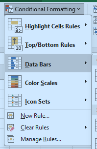
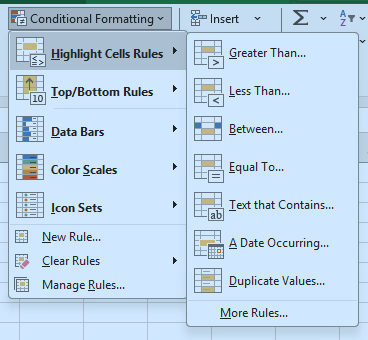
Under Highlight Cells Rules you can colour cells that are greater than, less than, between, equal to, containing certain text, or duplicated.
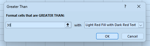
For example, Greater Than asks for a number and a colour. The cells update as you type.
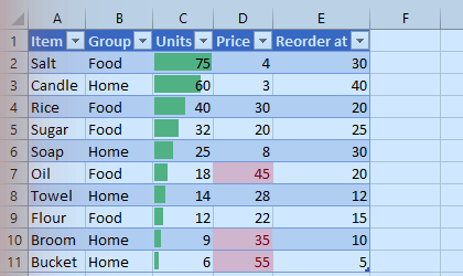
Conditional formatting changes a cell's appearance based on...
Flag a score of 60 or more as HIGH and everything else as -. Fill C2:C4.
Finish the quick check (and any code exercise) to complete this lesson, or mark it done yourself.
Tip: use the left and right arrow keys to move between lessons.